In the field of machine learning, the main objective is to find the most “fit” model trained over a particular task or a bunch of tasks. To do this, one needs to optimize the loss/cost function, and this will assist in minimizing error. One needs to know the nature of concave and convex functions since they are the ones that assist in optimizing problems effectively. These convex and concave functions form the foundation of many machine learning algorithms and influence the minimization of loss for training stability. In this article, you’ll learn what concave and convex functions are, their differences, and how they impact the optimization strategies in machine learning.
What is a Convex Function?
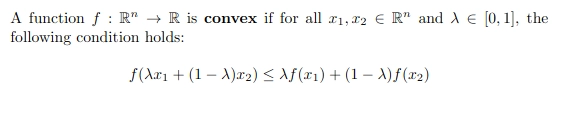
In mathematical terms, a real-valued function is convex if the line segment between any two points on the graph of the function lies above the two points. In simple terms, the convex function graph is shaped like a “cup “ or “U”.
A function is said to be convex if and only if the region above its graph is a convex set.

This inequality ensures that functions do not bend downwards. Here is the characteristic curve for a convex function:

What is a Concave Function?
Any function that is not a convex function is said to be a concave function. Mathematically, a concave function curves downwards or has multiple peaks and valleys. Or if we try to connect two points with a segment between 2 points on the graph, then the line lies below the graph itself.
This means that if any two points are present in the subset that contains the whole segment joining them, then it’s a convex function, otherwise, it’s a concave function.

This inequality violates the convexity condition. Here is the characteristic curve for a concave function:

Difference between Convex and Concave Functions
Below are the differences between convex and concave functions:
| Aspect | Convex Functions | Concave Functions |
|---|---|---|
| Minima/Maxima | Single global minimum | Can have multiple local minima and a local maximum |
| Optimization | Easy to optimize with many standard techniques | Harder to optimize; standard techniques may fail to find the global minimum |
| Common Problems / Surfaces | Smooth, simple surfaces (bowl-shaped) | Complex surfaces with peaks and valleys |
| Examples |
f(x) = x2, f(x) = ex, f(x) = max(0, x) |
f(x) = sin(x) over [0, 2π] |

Optimization in Machine Learning
In machine learning, optimization is the process of iteratively improving the accuracy of machine learning algorithms, which ultimately lowers the degree of error. Machine learning aims to find the relationship between the input and the output in supervised learning, and cluster similar points together in unsupervised learning. Therefore, a major goal of training a machine learning algorithm is to minimize the degree of error between the predicted and true output.
Before proceeding further, we have to know a few things, like what the Loss/Cost functions are and how they benefit in optimizing the machine learning algorithm.
Loss/Cost functions
Loss function is the difference between the actual value and the predicted value of the machine learning algorithm from a single record. While the cost function aggregated the difference for the entire dataset.
Loss and cost functions play an important role in guiding the optimization of a machine learning algorithm. They show quantitatively how well the model is performing, which serves as a measure for optimization techniques like gradient descent, and how much the model parameters need to be adjusted. By minimizing these values, the model gradually increases its accuracy by reducing the difference between predicted and actual values.

Convex Optimization Benefits
Convex functions are particularly beneficial as they have a global minima. This means that if we are optimizing a convex function, it will always be certain that it will find the best solution that will minimize the cost function. This makes optimization much easier and more reliable. Here are some key benefits:
- Assurity to find Global Minima: In convex functions, there is only one minima that means the local minima and global minima are same. This property eases the search for the optimal solution since there is no need to worry to stuck in local minima.
- Strong Duality: Convex Optimization shows that strong duality means the primal solution of one problem can be easily related to the relevant similar problem.
- Robustness: The solutions of the convex functions are more robust to changes in the dataset. Typically, the small changes in the input data do not lead to large changes in the optimal solutions and convex function easily handles these scenarios.
- Number stability: The algorithms of the convex functions are often more numerically stable compared to the optimizations, leading to more reliable results in practice.
Challenges With Concave Optimization
The major issue that concave optimization faces is the presence of multiple minima and saddle points. These points make it difficult to find the global minima. Here are some key challenges in concave functions:
- Higher computational cost: Due to the deformity of the loss, concave problems often require more iterations before optimization to increase the chances of finding better solutions. This increases the time and the computation demand as well.
- Local Minima: Concave functions can have multiple local minima. So the optimization algorithms can easily get trapped in these suboptimal points.
- Saddle Points: Saddle points are the flat regions where the gradient is 0, but these points are neither local minima nor maxima. So the optimization algorithms like gradient descent may get stuck there and take a longer time to escape from these points.
- No Assurity to find Global Minima: Unlike the convex functions, Concave functions do not guarantee to find the global/optimal solution. This makes evaluation and verification more difficult.
- Sensitive to initialization/starting point: The starting point influences the final outcome of the optimization techniques the most. So poor initialization may lead to the convergence to a local minima or a saddle point.
Strategies for Optimizing Concave Functions
Optimizing a Concave function is very challenging because of its multiple local minima, saddle points, and other issues. However, there are several strategies that can increase the chances of finding optimal solutions. Some of them are explained below.
- Smart Initialization: By choosing algorithms like Xavier or HE initialization techniques, one can avoid the issue of starting point and reduce the chances of getting stuck at local minima and saddle points.
- Use of SGD and Its Variants: SGD (Stochastic Gradient Descent) introduces randomness, which helps the algorithm to avoid local minima. Also, advanced techniques like Adam, RMSProp, and Momentum can adapt the learning rate and help in stabilizing the convergence.
- Learning Rate Scheduling: Learning rate is like the steps to find the local minima. So, selecting the optimal learning rate iteratively helps in smoother optimization with techniques like step decay and cosine annealing.
- Regularization: Techniques like L1 and L2 regularization, dropout, and batch normalization reduce the chances of overfitting. This enhances the robustness and generalization of the model.
- Gradient Clipping: Deep learning faces a major issue of exploding gradients. Gradient clipping controls this by cutting/capping the gradients before the maximum value and ensures stable training.
Conclusion
Understanding the difference between convex and concave functions is effective for solving optimization problems in machine learning. Convex functions offer a stable, reliable, and efficient path to the global solutions. Concave functions come with their complexities, like local minima and saddle points, which require more advanced and adaptive strategies. By selecting smart initialization, adaptive optimizers, and better regularization techniques, we can mitigate the challenges of Concave optimization and achieve a higher performance.
Hi, I’m Vipin. I’m passionate about data science and machine learning. I have experience in analyzing data, building models, and solving real-world problems. I aim to use data to create practical solutions and keep learning in the fields of Data Science, Machine Learning, and NLP.
Login to continue reading and enjoy expert-curated content.


