What is Beam Search in NLP Decoding?

Beam search is a powerful decoding algorithm extensively used in natural language processing (NLP) and machine learning. It is especially important in sequence generation tasks such as text generation, machine translation, and summarization. Beam search balances between exploring the search space efficiently and generating high-quality output. In this blog, we will dive deep into the workings of beam search, its importance in decoding, and an implementation while exploring its real-world applications and challenges.

Learning Objectives

• Understand the concept and working mechanism of the beam search algorithm in sequence decoding tasks.
• Learn the significance of beam width and how it balances exploration and efficiency in search spaces.
• Explore the practical implementation of beam search using Python with step-by-step guidance.
• Analyze real-world applications and challenges associated with beam search in NLP tasks.
• Gain insights into the advantages of beam search over other decoding algorithms like greedy search.

This article was published as a part of the Data Science Blogathon.

What is Beam Search?

Beam search is a heuristic search algorithm used to decode sequences from models such as transformers, LSTMs, and other sequence-to-sequence architectures. It generates text by maintaining a fixed number (“beam width”) of the most probable sequences at each step. Unlike greedy search, which only picks the most likely next token, beam search considers multiple hypotheses at once. This ensures that the final sequence is not only fluent but also globally optimal in terms of model confidence.

For example, in machine translation, there might be multiple valid ways to translate a sentence. Beam search allows the model to explore these possibilities by keeping track of multiple candidate translations simultaneously.

How Does Beam Search Work?

Beam search works by exploring a graph where nodes represent tokens and edges represent probabilities of transitioning from one token to another. At each step:

• The algorithm selects the top-k most probable tokens based on the model’s output logits (probability distribution).
• It expands these tokens into sequences, calculates their cumulative probabilities, and retains the top-k sequences for the next step.
• This process continues until a stopping condition is met, such as reaching a special end-of-sequence token or a predefined length.

Concept of Beam Width

The “beam width” determines how many candidate sequences are retained at each step. A larger beam width allows for exploring more sequences but increases computational cost. Conversely, a smaller beam width is faster but risks missing better sequences due to limited exploration.

Why Beam Search is Important in Decoding?

Beam search is vital in decoding for several reasons:

• Improved Sequence Quality: By exploring multiple hypotheses, beam search ensures that the generated sequence is globally optimal rather than being stuck in a local optimum.
• Handling Ambiguities: Many NLP tasks involve ambiguities, such as multiple valid translations or interpretations. Beam search helps explore these possibilities and select the best one.
• Efficiency: Compared to exhaustive search, beam search is computationally efficient while still exploring a significant portion of the search space.
• Flexibility: Beam search can be adapted to various tasks and sampling strategies, making it a versatile choice for sequence decoding.

Practical Implementation of Beam Search

Below is a practical example of beam search implementation. The algorithm builds a search tree, evaluates cumulative scores, and selects the best sequence:

Step 1: Install and Import Dependencies

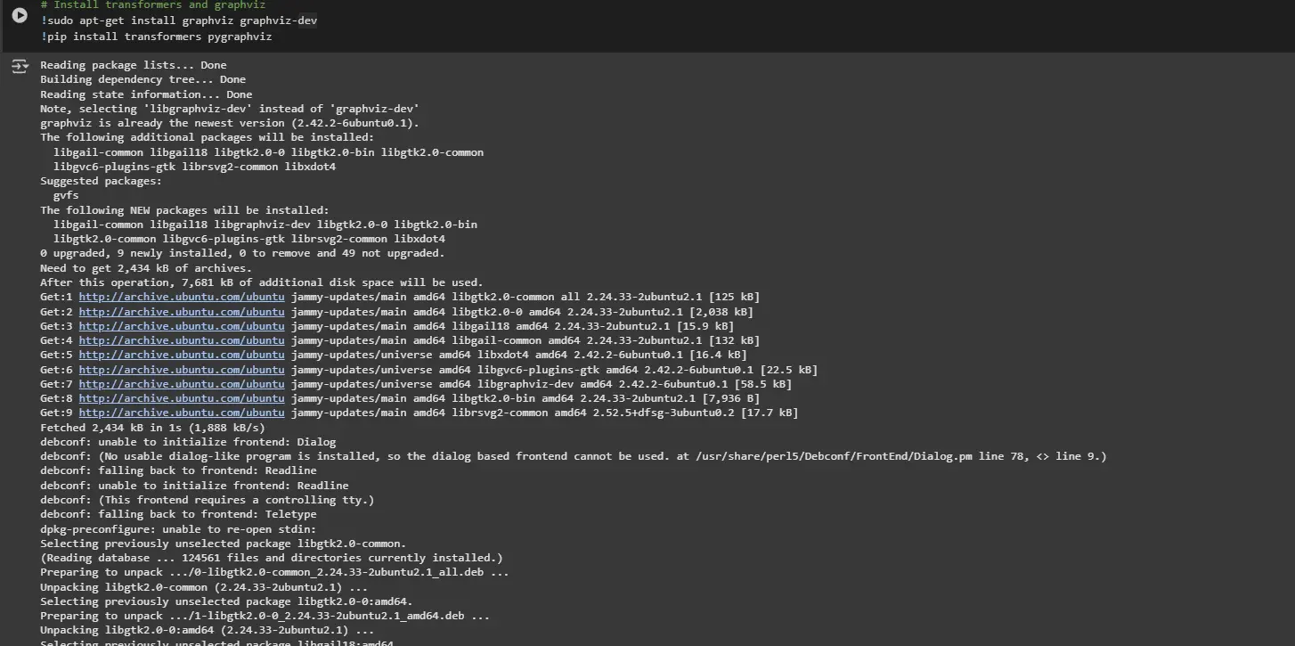
# Install transformers and graphviz
!sudo apt-get install graphviz graphviz-dev
!pip install transformers pygraphviz

from transformers import GPT2LMHeadModel, GPT2Tokenizer
import torch
import matplotlib.pyplot as plt
import networkx as nx
import numpy as np
from matplotlib.colors import LinearSegmentedColormap
from tqdm import tqdm
import matplotlib.colors as mcolors

System Commands: Installs required libraries for graph generation (graphviz) and Python packages (transformers and pygraphviz).

Imported Libraries:

• transformers: To load GPT-2 for text generation.
• torch: For handling tensors and running computations on the model.
• matplotlib.pyplot: To plot the beam search graph.
• networkx: For constructing and managing the tree-like graph representing beam search paths.
• tqdm: To display a progress bar while processing the graph.
• numpy and matplotlib.colors: For working with numerical data and color mappings in visualizations.

Output:

Step 2: Model and Tokenizer Setup

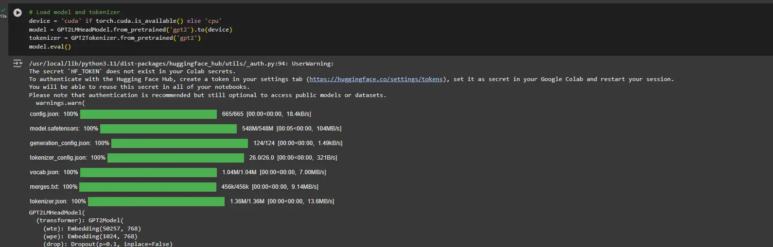
# Load model and tokenizer
device="cuda" if torch.cuda.is_available() else 'cpu'
model = GPT2LMHeadModel.from_pretrained('gpt2').to(device)
tokenizer = GPT2Tokenizer.from_pretrained('gpt2')
model.eval()

• Detects whether a GPU (cuda) is available, as it can accelerate computations. Defaults to cpu if no GPU is found.
• Loads the pre-trained GPT-2 language model and its tokenizer from Hugging Face’s transformers library.
• Moves the model to the appropriate device (cuda or cpu).
• Sets the model to evaluation mode with model.eval() to disable features like dropout, which are only needed during training.

Output:

Step 3: Encode Input Text

# Input text
text = "I have a dream"
input_ids = tokenizer.encode(text, return_tensors="pt").to(device)

• Defines the input text “I have a dream”.
• Encodes the text into token IDs using the tokenizer, returning a tensor (return_tensors=’pt’).
• Moves the input tensor to the appropriate device (cuda or cpu).

Step 4: Define Helper Function: Log Probability

def get_log_prob(logits, token_id):
    probabilities = torch.nn.functional.softmax(logits, dim=-1)
    log_probabilities = torch.log(probabilities)
    return log_probabilities[token_id].item()

• Applies the softmax function to convert logits into probabilities (distribution over vocabulary).
• Takes the natural logarithm of these probabilities to get log probabilities.
• Returns the log probability corresponding to the given token.

Step 5: Define Recursive Beam Search

Implements recursive beam search for text generation using the GPT-2 model.

def beam_search(input_ids, node, bar, length, beams, temperature=1.0):
    if length == 0:
        return

    outputs = model(input_ids)
    predictions = outputs.logits

    # Get logits for the next token
    logits = predictions[0, -1, :]
    top_token_ids = torch.topk(logits, beams).indices

    for j, token_id in enumerate(top_token_ids):
        bar.update(1)

        # Compute the score of the predicted token
        token_score = get_log_prob(logits, token_id)
        cumulative_score = graph.nodes[node]['cumscore'] + token_score

        # Add the predicted token to the list of input ids
        new_input_ids = torch.cat([input_ids, token_id.unsqueeze(0).unsqueeze(0)], dim=-1)

        # Add node and edge to graph
        token = tokenizer.decode(token_id, skip_special_tokens=True)
        current_node = list(graph.successors(node))[j]
        graph.nodes[current_node]['tokenscore'] = np.exp(token_score) * 100
        graph.nodes[current_node]['cumscore'] = cumulative_score
        graph.nodes[current_node]['sequencescore'] = cumulative_score / len(new_input_ids.squeeze())
        graph.nodes[current_node]['token'] = token + f"_{length}_{j}"

        # Recursive call
        beam_search(new_input_ids, current_node, bar, length - 1, beams, temperature)

• Base Case: Stops recursion when length reaches 0 (no more tokens to predict).
• Model Prediction: Passes input_ids through GPT-2 to get logits for the next token.
• Top Beams: Selects the beams most likely tokens using torch.topk().
• Token Scoring: Evaluates token probabilities to determine the best sequences.
• Extend Input: Appends the selected token to input_ids for further exploration.
• Update Graph: Tracks progress by expanding the search tree with new tokens.
• Recursive Call: Repeats the process for each beam (beams branches).

Step 6: Retrieve Best Sequence

Finds the best sequence generated during beam search based on cumulative scores.

def get_best_sequence(G):
    # Find all leaf nodes
    leaf_nodes = [node for node in G.nodes if G.out_degree(node) == 0]

    # Find the best leaf node based on sequence score
    max_score_node = max(leaf_nodes, key=lambda n: G.nodes[n]['sequencescore'])
    max_score = G.nodes[max_score_node]['sequencescore']

    # Retrieve the path from root to this node
    path = nx.shortest_path(G, source=0, target=max_score_node)

    # Construct the sequence
    sequence = "".join([G.nodes[node]['token'].split('_')[0] for node in path])
    return sequence, max_score

• Identifies all leaf nodes (nodes with no outgoing edges).
• Finds the best leaf node (highest sequencescore).
• Retrieves the path from the root node (start) to the best node.
• Extracts and joins tokens along this path to form the final sequence.

Step 7: Plot the Beam Search Graph

Visualizes the tree-like beam search graph.

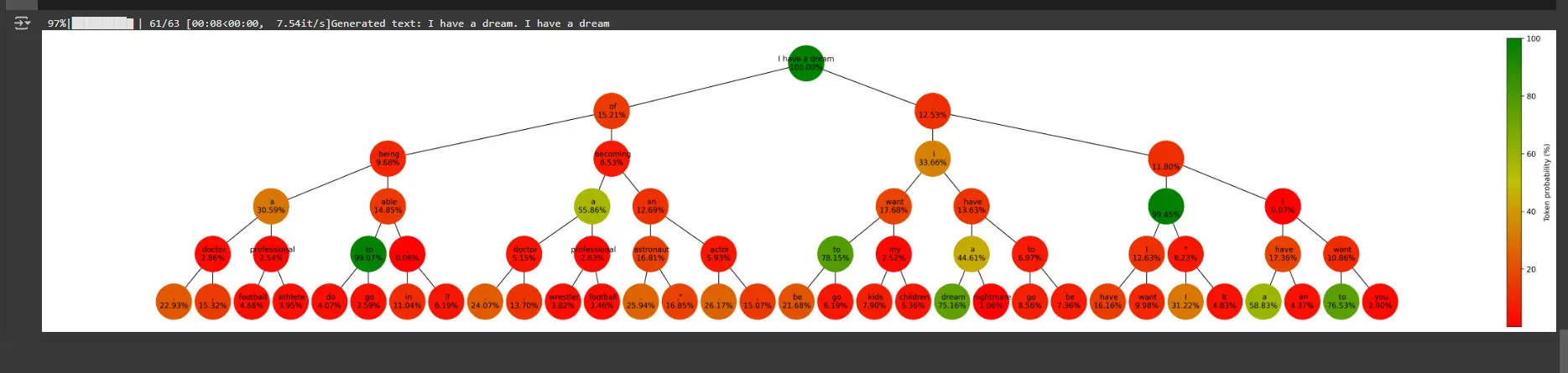
def plot_graph(graph, length, beams, score):
    fig, ax = plt.subplots(figsize=(3 + 1.2 * beams**length, max(5, 2 + length)), dpi=300, facecolor="white")

    # Create positions for each node
    pos = nx.nx_agraph.graphviz_layout(graph, prog="dot")

    # Normalize the colors along the range of token scores
    scores = [data['tokenscore'] for _, data in graph.nodes(data=True) if data['token'] is not None]
    vmin, vmax = min(scores), max(scores)
    norm = mcolors.Normalize(vmin=vmin, vmax=vmax)
    cmap = LinearSegmentedColormap.from_list('rg', ["r", "y", "g"], N=256)

    # Draw the nodes
    nx.draw_networkx_nodes(graph, pos, node_size=2000, node_shape="o", alpha=1, linewidths=4,
                           node_color=scores, cmap=cmap)

    # Draw the edges
    nx.draw_networkx_edges(graph, pos)

    # Draw the labels
    labels = {node: data['token'].split('_')[0] + f"\n{data['tokenscore']:.2f}%" \
              for node, data in graph.nodes(data=True) if data['token'] is not None}
    nx.draw_networkx_labels(graph, pos, labels=labels, font_size=10)
    plt.box(False)

    # Add a colorbar
    sm = plt.cm.ScalarMappable(cmap=cmap, norm=norm)
    sm.set_array([])
    fig.colorbar(sm, ax=ax, orientation='vertical', pad=0, label="Token probability (%)")
    plt.show()

• Nodes represent tokens generated at each step, color-coded by their probabilities.
• Edges connect nodes based on how tokens extend sequences.
• A color bar represents the range of token probabilities

Step 8: Main Execution

# Parameters
length = 5
beams = 2

# Create a balanced tree graph
graph = nx.balanced_tree(beams, length, create_using=nx.DiGraph())
bar = tqdm(total=len(graph.nodes))

# Initialize graph attributes
for node in graph.nodes:
    graph.nodes[node]['tokenscore'] = 100
    graph.nodes[node]['cumscore'] = 0
    graph.nodes[node]['sequencescore'] = 0
    graph.nodes[node]['token'] = text

# Perform beam search
beam_search(input_ids, 0, bar, length, beams)

# Get the best sequence
sequence, max_score = get_best_sequence(graph)
print(f"Generated text: {sequence}")

# Plot the graph
plot_graph(graph, length, beams, 'token')

Explanation

Parameters:

• length: Number of tokens to generate (depth of the tree).
• beams: Number of branches (beams) at each step.

Graph Initialization:

• Creates a balanced tree graph (each node has beams children, depth=length).
• Initializes attributes for each node:(e.g., tokenscore, cumscore, token)
  • Beam Search: Starts the beam search from the root node (0)
  • Best Sequence: Extracts the highest-scoring sequence from the graph
  • Graph Plot: Visualizes the beam search process as a tree.

Output:

You can access colab notebook here

Challenges in Beam Search

Despite its advantages, beam search has some limitations:

• Beam Size Trade-off
• Repetitive Sequences
• Bias Toward Shorter Sequences

Despite its advantages, beam search has some limitations:

• Beam Size Trade-off: Choosing the right beam width is challenging. A small beam size might miss the best sequence, while a large beam size increases computational complexity.
• Repetitive Sequences: Without additional constraints, beam search can produce repetitive or nonsensical sequences.
• Bias toward Shorter Sequences: The algorithm might favor shorter sequences because of the way probabilities are accumulated.

Conclusion

Beam search is a cornerstone of modern NLP and sequence generation. By maintaining a balance between exploration and computational efficiency, it enables high-quality decoding in tasks ranging from machine translation to creative text generation. Despite its challenges, beam search remains a preferred choice due to its flexibility and ability to produce coherent and meaningful outputs.

Understanding and implementing beam search equips you with a powerful tool to enhance your NLP models and applications. Whether you’re working on language models, chatbots, or translation systems, mastering beam search will significantly elevate the performance of your solutions.

Key Takeaways

• Beam search is a decoding algorithm that balances efficiency and quality in sequence generation tasks.
• The choice of beam width is critical; larger beam widths improve quality but increase computational cost.
• Variants like diverse and constrained beam search allow customization for specific use cases.
• Combining beam search with sampling strategies enhances its flexibility and effectiveness.
• Despite challenges like bias toward shorter sequences, beam search remains a cornerstone in NLP.

Frequently Asked Questions

The media shown in this article is not owned by Analytics Vidhya and is used at the Author’s discretion.

I’m Neha Dwivedi, a Data Science enthusiast , Graduated from MIT World Peace University,Pune. I’m passionate about Data Science and rising trends with it. I’m excited to share insights and learn from this community!